Import a Data Hierarchy from Excel into SQL Server
When a client hands you data for a project, it's usually in a database of some kind. Today, I'll demonstrate how to work some Excel magic to import a hierarchy into a database.

Lately, I've been taking on a lot of work with a couple of clients.
After talking with one client, he mentioned how he was working with his data and provided me an Excel spreadsheet.
Wait a minute?!?! Did they just say "Excel spreadsheet" for managing his data?
While I can understand Excel is what most people have at the time, it's definitely not a database.
I know Excel has the option to save as CSV, but we have a problem with this particular issue.
The data looks like this (NOTE: I'm using mocked up data to protect the project).
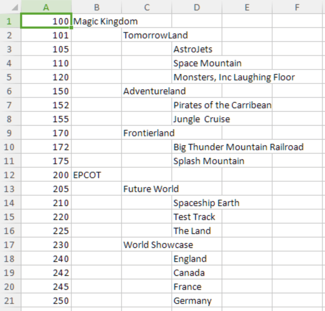
As you can see, this really isn't a great CSV format to work with when exported. This usually requires some massaging of data before the data can be usable.
Do everything you can inside of Excel to make it a little more usable. Why?
Because I'm sure in the future, they'll give you an updated Excel file and expect you to import it just as quick.
To give you an idea of what our final table looks like, it'll look similar to our menu system from earlier this year.
A couple of issues include:
- I need a parent ID for the children so I can identify how deep is this hierarchy.
- A level indicator would be a great indicator for determining parent-children relationships.
- We need to flatten the data so we can work with it.
- Finally, the data does need to be in a CSV to import into SQL Server.
So let's flatten this hierarchy so it's usable!
Flatten the Data
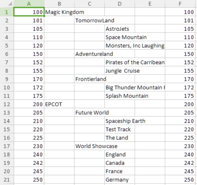
First, I want to copy over the Unique ID in A1 to keep the data clean. So it's a simple "=A1" formula in Column F.
Copy the cell and paste it all the way down to "Germany."
Your spreadsheet will look like this.
This next part took a little detective work to find this Excel gem.
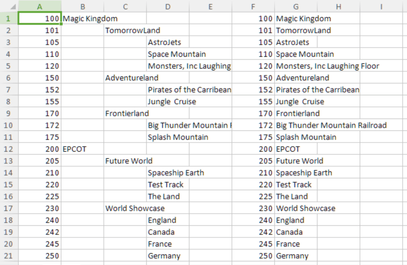
In this next step, we need to remove all of the columns that have space and place the text in Column G.
The INDEX/MATCH duo works absolute wonders for this type of processing.
In G1, type:
=INDEX(B1:D1,MATCH(TRUE,INDEX((B1:D1<>0),0),0))
Let's break this down.
The INDEX((B1:D1<>0),0) checks to see if there is anything in cells B1, C1, or D1 and returns the number.
The MATCH looks for the text at that location returned from the INDEX.
Finally, the outer INDEX returns the actual value based on the MATCH returning Magic Kingdom to the cell.
Copy that formula and all of your hierarchy will be flattened!
Sledgehammer It!
To get the level of the hierarchy, I used a simple numbering system for it.
=IF(ISBLANK(B1),IF(ISBLANK(C1),IF(ISBLANK(D1),3,2),1),0)
Copy and paste this formula into Column H.
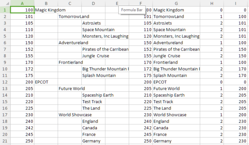
We now have our hierarchy levels.
The Hard Part
Determining the parent id was something I spent a loooong time trying to figure out.
How do you get the parent value of a cell when you are sitting at the child level?
The only way I solved this was to use the spaces in the hierarchy to my advantage.
Here's the $10,000 line of code to perform the lookup.
=IF(H1=0,0,IF(H1=1,INDEX($A$1:$A$21,MATCH("*",$B$1:B1,-1)),IF(H1=2,INDEX($A$1:$A$21,MATCH("*",$C$1:C1,-1)))))
Ok, yes, it's a bit intimidating, but once you break it down, it makes sense.
Based on the current row I'm on, I check the level number.
- If I'm at level 0, ignore it. It's zero, or null or whatever we want to use for our root number.
- If I'm at level 1, I know that the parent is located in Column B in a non-empty cell from my current location (current row/column B) going up the chain until I hit a non-empty cell (Magic Kingdom).
- If I'm at level 2, execute the same process, but instead, check Column C from the current row on up to a non-empty cell.
The INDEX/MATCH combination provided me with the ID once the MATCH found the non-empty cell using the INDEX($A$1:$A$21... range. Once it found the match, it placed the unique ID into Column I.
Copy and paste that "down to Germany" and your spreadsheet should now look like this.
For more information on the INDEX/MATCH combo, check out AbleBits. They have a great write-up on INDEX/MATCH with examples on how to maximize your lookups...without VLOOKUP!
Conclusion
You can now take those columns from Column F-I (minus the Column H/levels) and save the file as a CSV file to import into SQL Server.
You also have a simple way to copy and paste the formulas to flatten your structure for your database of choice.
Have you ever dug this deep into Excel? Did this solve a problem for you? Post your comments below and let's discuss.


